RTP estimation fundamentals#
The round-trip phase (previously known as PDE) is a technique that utilizes the phase difference between an MD (which is the initiator) and determines the need to estimate distance and an active RD to determine the distance between them.
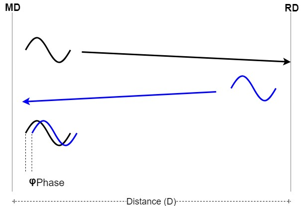
In its simplest form, the MD transmits a continuous wave to the RD, which synchronizes its phase and sends the signal back to the MD. The MD then compares the phase of the received signal with the phase of the signal it transmitted, obtaining a phase difference.
Phase difference using an MD and an RD
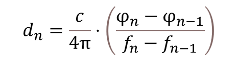
With this information, the distance can be measured using the following equation:
Equation 11. Measure distance using a single-phase difference

Where:
φ is the phase difference, as measured by MD.
c is the speed of light.
f is the carrier frequency.
n is the number of wraps.
Note that the number of wraps (n) depends on the wavelength of the carrier frequency.
Equation 12. Wavelength of the carrier frequency

If the distance to measure is larger than λ, the phase wraps (creating a distance ambiguity) and the number of wraps (n) must be accounted for.
A sweep of multiple frequencies is used to reduce the above-mentioned ambiguity and to aid in analyzing multipath scenarios. If the phase difference is obtained at two different frequencies and the equations are combined, the following equation can be used to determine the distance:
Equation 13. Distance estimation using two frequencies

Slope-based PDE#
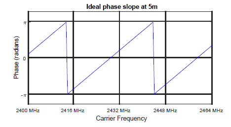
If a frequency sweep is done at a fixed distance and with constant spacing between the frequencies (Δf), the phases obtained at each frequency in the sweep produce a slope.
Phase slope at 5 m
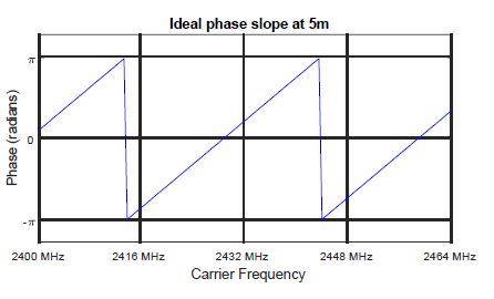
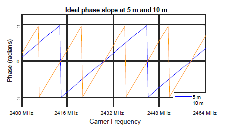
There is a linear relationship between the phase slope observed and the distance to the object. The smaller the slope, the shorter the distance between RD and MD.
Phase slope difference at 5 m and 10 m
Using this slope, the equivalent distance can be obtained using the following equation:
Equation 14. Distance obtained from phase slope

To get the slope-based distance using phase differences obtained at several frequencies, Equation 13 must be applied multiple times, as shown in the following equation:
Equation 15. Immediate distance from a single-phase difference
The final distance estimate can be obtained as follows:
Equation 16. Distance obtained from the average of immediate distances

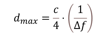
The maximum measurable distance depends on the spacing between the measurement frequencies (Δf) and it is given by the following equation:
Equation 17. Maximum distance measurable using the slope method
Parent topic:RTT estimation fundamentals
Complex Distance Estimation (CDE)#
In CDE, the phase measurements taken at each frequency are converted into a complex signal in the frequency domain. By transforming it to the time domain using the Inverse Fast Fourier Transform (IFFT), we obtain the distribution of the propagation delays that are in the signal.
The maximum propagation delay that can be measured without ambiguity is determined by the spacing between the measurement frequencies (Δf) and it is given by the following equation:
Equation 18. Largest unambiguous propagation delay measurable using the CDE method

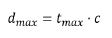
The maximum measurable distance can be obtained by multiplying the maximum propagation speed by the speed of light (c):
Equation 19. Maximum distance measurable using the CDE method
The distance estimate is obtained using the following equation:
Equation 20. CDE distance calculation
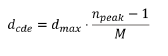
Where npeakis the bin with the highest peak, M is the number of bins used in the IFFT, and dmax is the largest unambiguous distance. Let’s assume an ideal phase difference response for two boards separated by 5 m. The phase difference is measured using Δf = 500 kHz. The maximum measurable distance is given by the following equation:
Equation 21. Maximum distance measurable using Δf = 500 kHz

The wrapped phase response obtained from the frequency sweep at the same distance (see Figure 20) is shown in Figure 22.
Ideal phase slope at 5 m using Δf = 500 kHz

If a 128-bin FFT is applied to an array containing the wrapped phase points in their rectangular form, the output is shown in Figure 23.
Ideal 128-bin IFFT for the 5-m slope
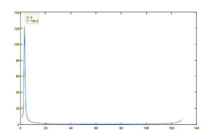
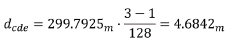
The bin holding the biggest peak is number 3. Use the following equation to obtain the estimated distance:
Distance calculation for bin 3 using 128-bin FFTe
The resolution of the measured distance depends on the frequency step selected and the number of bins used in the IFFT.
Parent topic:RTP estimation fundamentals
PDE implementation#
A two-way PDE estimation algorithm typically requires precise acquisition of phase changes across a span of frequencies by each participating device. The phases are derived from the captured I and Q samples in the receiver of a device for a tone transmitted by the peer device with a known raster.
The PDE implementation mainly consists of four steps: initialization and calibration, IQ data capture, phase processing, and distance estimation.
Initialization and calibration#
Before capturing the IQ samples, four important conditions must be met:
All transceiver impairments that can impact the phase capture information (DC offsets, IQ mismatch, filtering transfer function contributions, PLL phase excursions, and so on) must be minimized.
Theoretically, the IQ signal amplitude does not affect the phase calculations. However, signal saturation or fading can affect the accuracy of phase calculations. Ensure a good dynamic range for the captured IQ samples.
The measurement of phase differences implies that changes in phase are only produced by the distance between the test devices. The PLLs in both devices must remain frequency-coherent throughout the capture process.
Some algorithms require changing the tone frequencies with a specific time interval. The devices must synchronize their transmit and receive cycles accordingly.
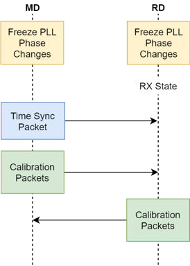
The initialization and calibration stages ensure that all of the above conditions are met before capturing the IQ samples.
Initialization and calibration sequence
Parent topic:PDE
IQ data capture#
Two-way PDE algorithms use multiple phase differences obtained at several frequencies. To achieve this, the MD and RD must generate Continuous-Wave (CW) tones and capture IQ samples in all the measurement frequencies.
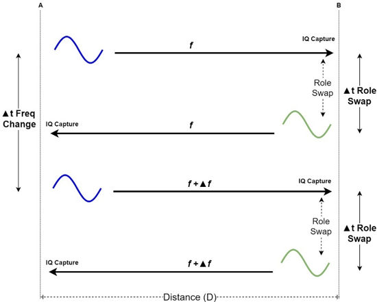
The base mechanism consists of device A, which generates a tone at frequency f. At the same time, the peer device B sets its radio to the RX mode at f and starts to capture IQ samples. After a fixed amount of time, devices A and B change roles. Now device B generates a tone in f and device A starts the RX and IQ capture at f. This is a tone exchange sequence.
After the tone exchange sequence ends, both devices return to their original roles, but the frequency is updated by Δf. For this new tone exchange, device A generates a tone at f + Δf. Device B also sets its radio to the RX mode at f + Δf and captures IQ samples. The tone exchange sequence is repeated for all frequency values that are defined for this measurement
Multiple frequency IQ samples capture sequence
Parent topic:PDE
Phase processing#
After the IQ samples are captured on each device, the phase difference is obtained using the following equation:
Equation 22. Phase from IQ samples

Each device holds the phase difference slope of the peer device against its own local oscillator. To obtain the phase combination result of the distance, the phase slope from the RD must be added to the phase slope from the MD.
Equation 23. Phase vector combination

This phase slope can now be used to perform distance estimation. As shown in Figure 21, depending on the frequencies used and the measured distance, phase wraps may occur.
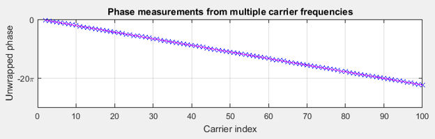
Figure 27 shows how the measured phase values change as a function of the carrier-frequency index. The data for this example is obtained using a wired setup, where the two devices are connected by a cable. A total of 99 carriers are used with the first carrier (index 2) corresponding to a frequency of 2400.5 MHz. The last carrier (with index 100) corresponds to a frequency of 2449.5 MHz. The frequency step size is 500 kHz.
Phase measurements (unwrapped) across multiple carrier frequencies

Parent topic:PDE
Distance estimation#
After the IQ samples are captured on each device, the phase difference is obtained using the following equation:
The phase vector obtained as a result of phase processing is the input for the distance-estimation algorithm. It can be used directly with Equation 16 for the slope method or as an IFFT input for the CDE method.
IFFT of phase vector
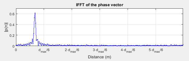
Figure 28 shows the IFFT magnitude response of the phase vector illustrated in Figure 27. The labels on the x-axis show the distance in meters. The final estimate is generally obtained from the peak location of the IFFT. The zero-meter compensation may be necessary to account for the delays within the radio front end.
Parent topic:PDE
Parent topic:RTP estimation fundamentals