RTT estimation fundamentals#
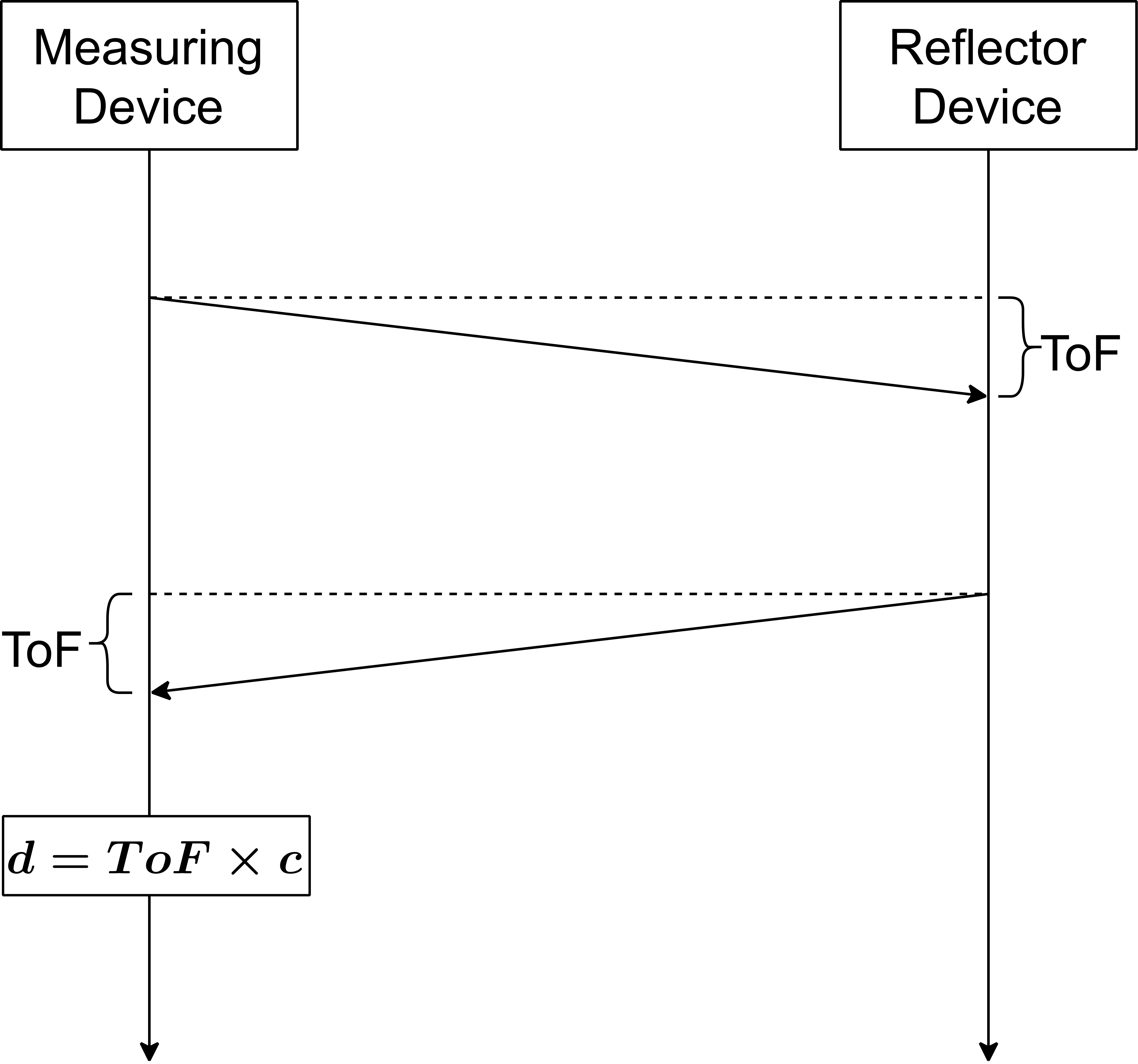
The round-trip time (previously known as the time of flight) is a method to measuring the distance between a sensor and an object, based on a precise measurement of the time difference between the transmission of a signal by the sensor and its return to the sensor after being reflected by an object. This approach is part of the RTT measurement. Wireless ToF applies the same concept to two wireless devices that can perform distance measurement between them by exchanging packets and accounting for radio latencies and turn-around time overheads.
The narrowband ToF requires at least two devices with NBW radio support to exchange packets over the air. As shown in Figure 13, it is based on a record of times at which the initial packet was transmitted by the MD and the time at which a response packet is received from the RD by the MD. The MD can calculate a ToF of the packet exchange. Using the calculated ToF, a distance estimate (or range) between the two devices can be computed. The determined distance (d) can be employed for a variety of functions, such as taking a specified action when the distance is above or below a threshold.
Basic ToF sequence

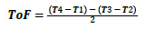
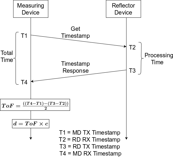
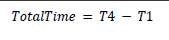
As shown in Figure 13, a method to capture the timestamps at which the packets are transmitted and received is required at both ends. Furthermore, these timestamps must be shared from RD to MD for the ToF calculation. The MD records a count from a timer (designated T1) in response to initiating transmission of the ranging packet. In response to receiving the ranging packet, the RD records a count from a local timer (designated T2). The RD takes a certain amount of time to process the incoming packet and send a response packet. This time is designated as “Processing Time”, which is an overhead that must be eliminated to get an accurate ToF reading. In response to initiating the transmission of the response packet, the RD stores the count (designated T3). The response packet includes a data payload indicating the timestamps to calculate the RD processing time. Upon receiving the response packet, the MD records the count (designated T4). With these timestamps, a ToF value can be generated according to Equation 1..
Calculation of ToF
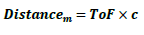
Once the ToF value is calculated, the distance can be estimated using Equation 2..
Distance estimation using ToF

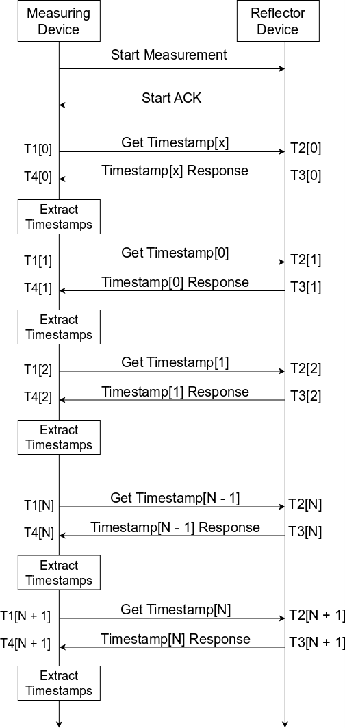
Figure 14 shows the sequence of packet exchange and timestamp collection for a single measurement.
ToF calculation using timestamps

Narrowband ToF#
Radio frequency waves travel at the speed of the light (c), which is a known constant (c ≈ 3×10⁸m/s); 1 m is equivalent to ~3.3 ns. A system measuring the ToF would ideally require a high-speed clock (GHz) to generate the timestamps with 1-ns accuracy, which is not possible with today’s low-cost deep submicron technologies. For mass-market applications, where low power consumption, low system complexity, and a tight cost budget are a constraint, a low-cost MCU with an integrated 2.4-GHz radio can be used. Typically, these devices work with a high-accuracy reference clock (Fref). As an example, using a reference clock of 32 MHz provides raw ToF accuracy of about 10 m, which may be adequate to validate a more precise but spoofable distance measurement. However, 10 m is too coarse and might not be useful as most applications require accuracy that is much finer. A typical target is to have accuracy of less than 1–2 m. To achieve such accuracy, a number of ToF measurements may be taken (approximating a normal distribution) and averaged. When using ToF distance estimation, there is a trade-off between accuracy and measurement time.
A narrowband ToF measurement systems consists of the following:
Counter for timestamping that is synchronized to the radio subsystem clock reference (Fref)
Precise hardware-based timestamping mechanism
Measurement protocol that includes the following steps:
Timestamp collection
Preprocessing
Postprocessing
Measurement report
Timestamping mechanism#
A precise timestamping mechanism is required on both ends for the NBW ToF to achieve the targeted accuracy. At the system level, this not only imposes requirements on the stability and relative accuracy of the timestamping clocks used by both MD and RD, it is also desired that the timestamp-capture mechanism does not contribute to additional jitter. This requirement typically implies that timestamping must be hardware-based and utilize precise triggers for both packet transmission and reception.
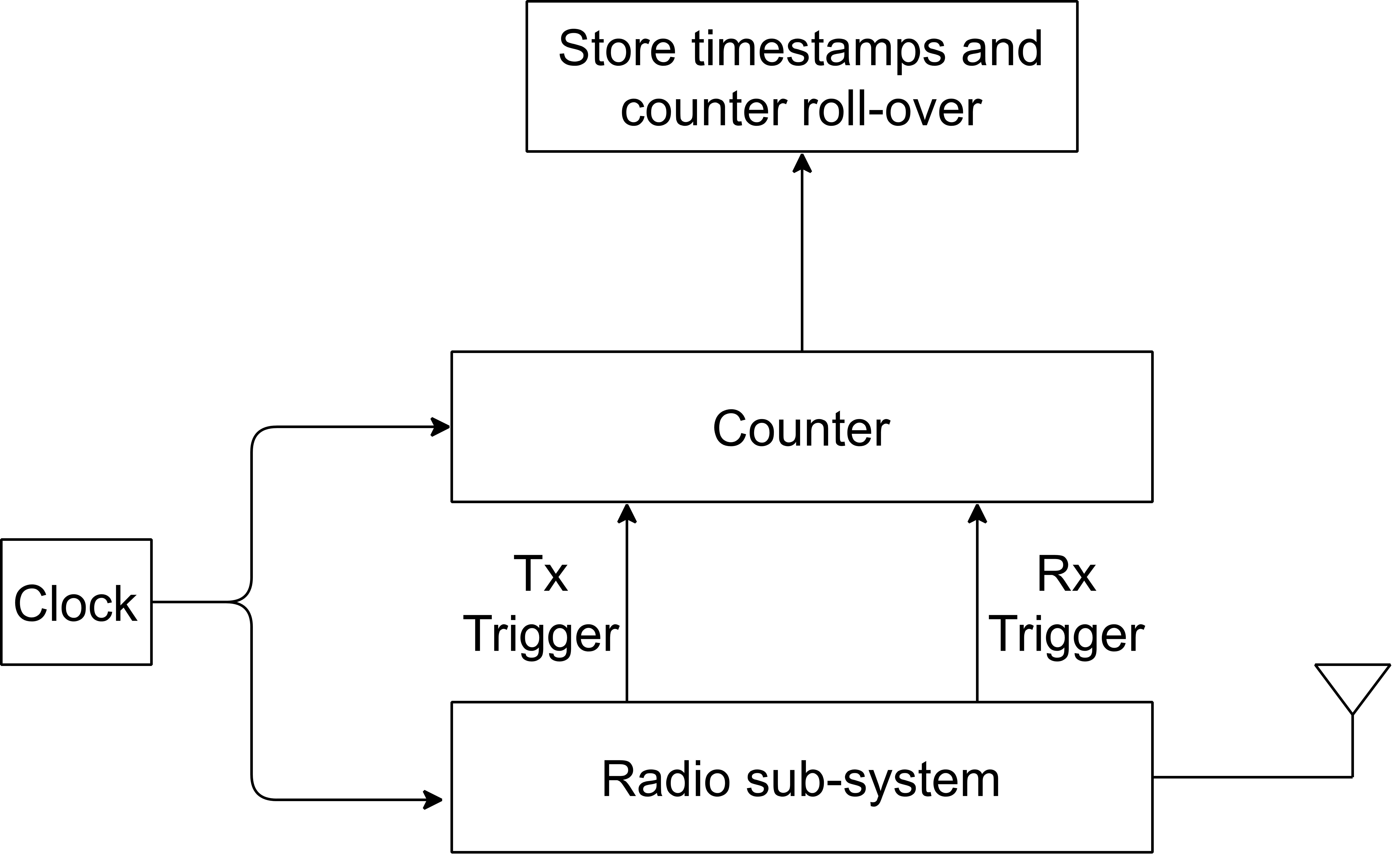
To generate precise timestamps, a deterministic and accurate counter is required. For instance, a 16-bit MCU timer, clocked by the radio’s reference clock, can be chosen. Given the counter-clock frequency and its size, the count overflows and roll-overs happen every few milliseconds, which must be accounted for as well. The timestamp trigger should be generated from the radio SoC to ensure a stable trigger at specific anchors of the packets. For instance, the transmission timestamp source could be taken from a signal asserted when the system is ready to transmit the first preamble bit. On the receiving end, a packet-reception trigger source can happen when the radio detects the synchronization delimiter (such as the access address in Bluetooth LE or Start-of-Frame Delimiter (SFD) for IEEE 802.15.4) arrival for the packet. Figure 15 shows the timestamp block diagram.
Timestamp block diagram

Parent topic:Narrowband ToF
Multi-stage ToF#
The ToF measurement consists of four stages: timestamp collection, preprocessing, postprocessing, and measurement report
ToF stages
Timestamp collection#
During this stage, the devices perform a series of packet exchanges. Each exchange creates a set of timestamps T1 – T4, which are made available to the MD for analysis. As T2 and T3 are generated at RD, they shall be shared on the response packet along with other information that might be useful, such as RSSI. As T3 (RD TX Timestamp) is generated by a transmission of the response packet, a causal implementation is possible by having the RD response to the MD contain timestamps corresponding to the previous packet exchange, as shown in Figure 17.
Wireless communication, especially in the shared Industrial, Scientific, and Medical (ISM) frequency band can be hampered by interference due to proximity of other radios utilizing the same frequency band and/or multi-path propagation artifacts. Using multiple carrier frequencies for ToF can reduce the impact of such artifacts and increases the likelihood of a successful ToF measurement. As explained in this document, a ToF distance measurement typically comprises of exchanging a set of packets for physical ToF measurements (by timestamping) as well as control communication between the two wireless nodes. Due to interference and artifacts, any of the packets containing either the timestamp requests, timestamped measurements, or measurement command packets might fail to arrive in either direction. For robust operation, a ToF measurement system should incorporate a robust mechanism that can recover from such events. Such a mechanism must be intelligent enough to identify and skip specific carrier frequencies if they have persistent interference and continue with the measurement on a different frequency, rather than just abort due to the missed packets.
Timestamping collection

Parent topic:Narrowband ToF
Preprocessing#
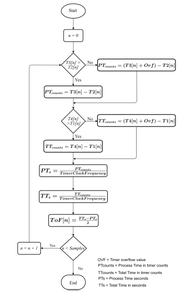
With the timestamps already generated and stored at MD, the pre-processing stage calculates a ToF estimate for every T1 – T4 sample set. Such calculations can be performed using integer math. However, to improve the measurement accuracy, fixed-point or floating-point math can be used. To calculate each ToF estimate, the system performs the following steps:
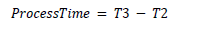
Calculate the process time in function of timer counts. Any timer overflow must be accounted in Equation 3.
Equation 3. Process time calculation
Calculate the total time in function of timer counts. Any timer overflow must be accounted in Equation 4.
Equation 4. Total time calculation

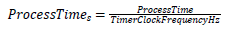
Translate the process time from TimerClockFrequencyHz counts to seconds, as shown in Equation 5.
Equation 5. Process time to seconds
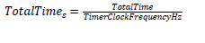
Translate the total time from TimerClockFrequencyHz counts to seconds, as shown in Equation 6.
Equation 6. Total time to seconds
Calculate the ToF per sample, as shown in Equation 7.
Equation 7. ToF in seconds
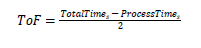
Figure 18 shows the previously discussed steps for n samples.
Individual ToF measurement and preprocessing flowchart

For a radio, it is typical to exercise the receiver’s Automatic Gain Control (AGC) dynamic range to operate over the entire link budget or in response to the presence of interference. The AGC operation typically ensures that a certain level of down-converted signal is maintained at the receiver’s Analog-to-Digital Conversion (ADC) over the receiver’s entire dynamic range, until the receiver gain hits either a minimum or a maximum. Since the measurement resolution targeted in the ranging-distance estimates is in nano-seconds, any propagation time variability within the radio’s analog front end due to gain adaptation must be carefully treated as a potential source of error, while performing the ToF distance estimation. This can be avoided by either performing a gain vs time propagation variability calibration. This can be addressed by choosing a robust method to choose an optimal AGC setting for a ToF measurement.
Parent topic:ToF Multistage
Postprocessing#
The postprocessing step is typically applied over a set of individual ToF measurements with a goal to choose a reliable distance estimate from several single-shot measurements that may be individually lacking both accuracy and resolution. Statistical estimation techniques must be applied in this step to the collected data set. As an example, the postprocessing step can include data-processing techniques, calculation of a statistical average (ToFaverage, mean or median), weighted averages, and so on. It may include statistical tests for outlier rejection (among others) to improve ToF accuracy.
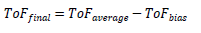
To cancel systematic delays in a ToF measurement, one option is to perform a calibration to estimate the bias that must be subtracted from ToFaverage. Such bias method can be carried out at a fixed distance between the two nodes. ToF is given as Equation 8.
Equation 8. ToF after bias
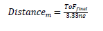
When a ToFfinal value is calculated, the distance between the two wireless nodes may be estimated by dividing ToFfinal by the ideal ToF value expected for a reference distance of 1 m (Equation 9).
Equation 9. Distance estimation

The measurement report is created when the calculated distance estimate is ready. The measuring device reports the estimated distance and an indication that the measurement is complete.
Parent topic:ToF Multistage
Zero distance calibration (ToFbias)#
The ToF calculation must account for any systematic offsets in the calculation, which may be contributed by the specific choice of receive and transmit trigger anchors in the exchanged packets, as well as radio-specific implementation, such as data path latencies, delays, and so on. This systematic offset in ToF computations may be eliminated via characterization or calibration.
For both the transmitted and received packets, the location of the anchor points in the packet that are timestamped are known. Combining this knowledge of anchor triggers to the ToF packet format and communication data rate, the theoretical time delay between a packet transmission by a device and its reception by another device for a known reference distance could be precisely computed if the data path latencies in the transceiver chain were negligible or precisely known. For ToF distance estimation, the timing resolution that must be resolved is in nanoseconds. This requires a reference physical measurement to have a precise measurement of the Radio Frequency (RF), analog and digital data path latencies, as well as other implementation delays in the control path.
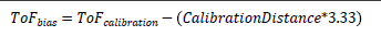
For this purpose, a calibration method is implemented by placing both devices (MD and RD) at a known distance and perform average ToF measurements over a set of exchanged packets. This enables the computation of averaged ToFbias, which is calculated according to Equation 10.
Equation 10. ToF bias

The ToF measurement is also impacted by propagation delay variation in the RF/analog front end of the radio as a function of the Automatic Gain Control (AGC) step in use. It is recommended to perform the ToF zero-distance calibration at a known distance and gain the configuration of the radio. For a random distance measurement using ToF, the knowledge of the receiver’s gain during the measurement and its relationship to the gain value used during the zero distance calibration may be used to compensate for the subsequent ToF measurements.
Parent topic:ToF Multistage
Parent topic:Narrowband ToF
Parent topic:RTT estimation fundamentals